Introduction
The UK’s energy grid needs help. Sometimes we generate too much renewable energy, and we have nowhere to put it, or we can’t move it to somewhere where it needs to go.
This doesn’t sound like a problem, except having “extra electricity” flowing around the grid is bad. There a few ways to fix this, and one of them is called curtailment. This is the official term for saying “let’s turn the renewables off for a bit”.
In 2021, we lost around £500m of electricity from windfarms due to curtailment. I’ve seen (unpublished) estimates that the problem in 2022 was significantly worse.
The grid works really hard to maintain balance between energy demand and energy supply. Sometimes, this results in curtailment. But what could we do differently? At PT1, we believe in finding and investing in the best energy storage startups. If you’re working on something in this field, get in touch and connect with me on LinkedIn.
I want to understand how energy storage could simplify the grid and prevent curtailing. In this post, I build a toy model to simulate an energy storage system, and then see what that implies for the ideal UK system.
Sections
- Toy Model
- Real world scenario
- Takeaways
Toy Model
We know that UK energy demand on an hourly basis is variable. We can also assume that the grid is perfectly balanced (generation = demand). In our toy model, we assume the demand/generation curve has a morning peak and then decreases.
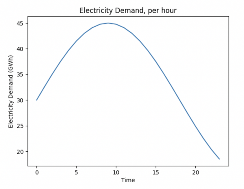
This demand variability is met by flexing our generation and ensuring the two are aligned as closely as possible. IE, if demand drops the grid will work to decrease generation (curtailment). If the demand increases the grid will try to increase generation by getting power providers to up their production.
Alternatively, we could have a constant energy generation (our baseline) alongside a perfect storage system. We could store the energy when demand is less than the baseline, and use that stored energy when demand outstrips the generation. This could stop curtailment entirely.
With our simulated system, let’s now add a baseline generation.
The baseline generation is found by finding the total daily energy demand, and then averaging it out. We can then show the daily behaviour of this energy storage system – it charges itself up at night, and discharges at the day time.
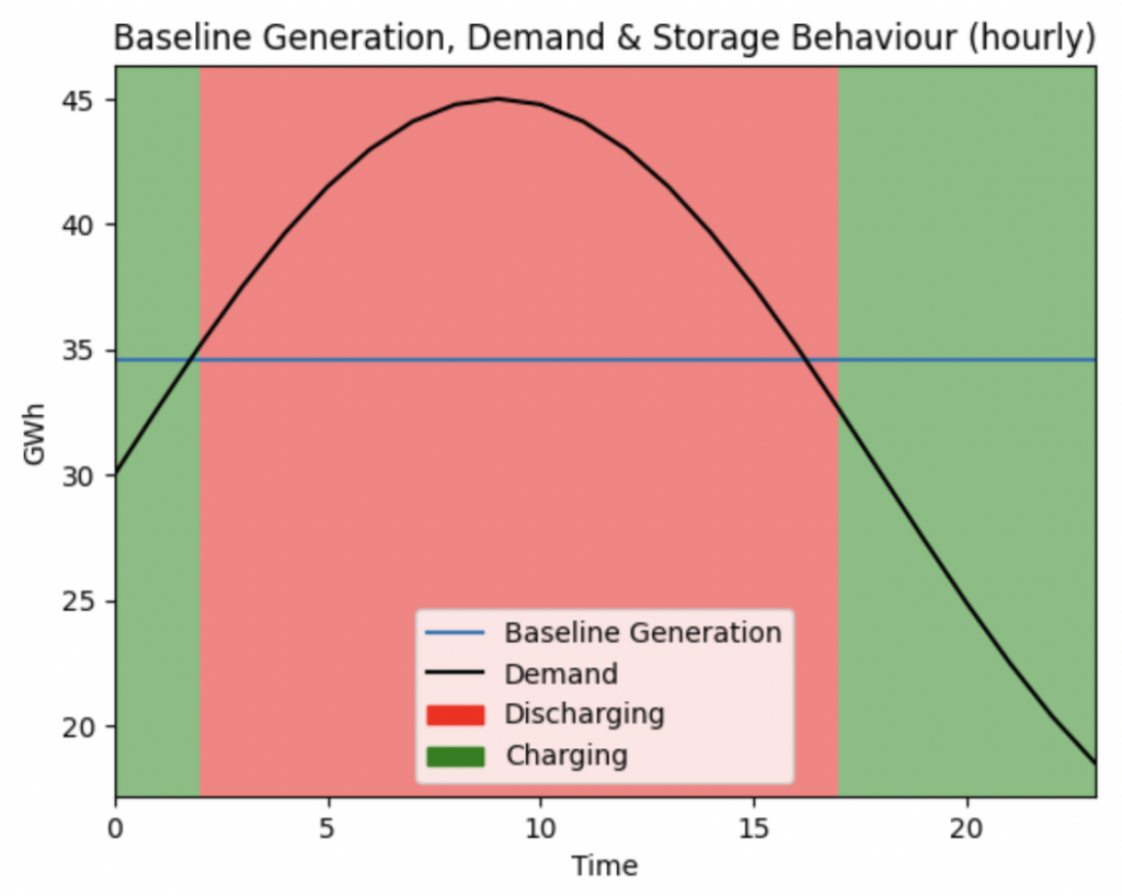
Again, this is with fake data – we may see different behaviour when we start to use real data for this. The red colour extends beyond the intersection point at ~16.00. This is a temporal aliasing issue as I’m using a low granularity timeframe.
Now, we can take a look at the behaviour of our storage system in more detail. This toy model consumes ~830 GWh of energy each day, which is comparable to the UK’s average daily consumption.
We get a baseline capacity of about 35 GWh.
We can find the total storage required (how much energy do we need in the red region), and that comes to 95 GWh.
These numbers form the physical constraints behind this system. The other values that matter are the charge and discharge rates. These show how quickly we need to add or remove energy from our storage system. A real world analogy would be storing energy by pumping water into a higher reservoir. There is a maximum amount of water we can pump each second, and that would be our charge rate. If the charge rate in the theoretical system exceeds the charge rate of a pumped water storage system, we know we need a better way of storing energy.
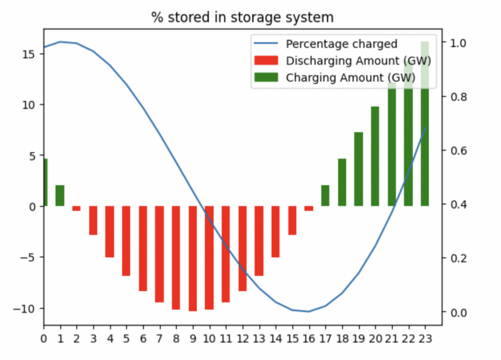
The storage curve above shows the percentage charged (in the storage system) throughout the day. I have given it a headstart, so it starts each day with enough energy to last. The maximum charge rate/ discharge rate are where the blue line is steepest, and also corresponds to the turning points of the bar chart.
From this toy model, we have max charge/ discharge rates of 16 GW and -10 GW.
So we have 4 key values which drive the model specification – baseline generation, storage capacity, maximum charge rate and maximum discharge rate.
Real world scenarios
In my toy model, I took a vaguely sinusoidal function as our demand and worked from there. Now, I’m going to use real UK demand data and run the exact same process to see what I get.
Using the National Grid’s Balance Mechanism Reporting System, I can get the half hourly demand forecast for the next 48 hours. Taking an average gives me a realistic picture of the UK’s usage (albeit in January, and therefore higher than our average 830 GWh from above).
It looks like:
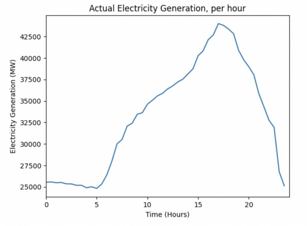
Now let’s apply the same logic to it as before. We analyse the UK generation curve, understand what the baseline should be and show how it should look:
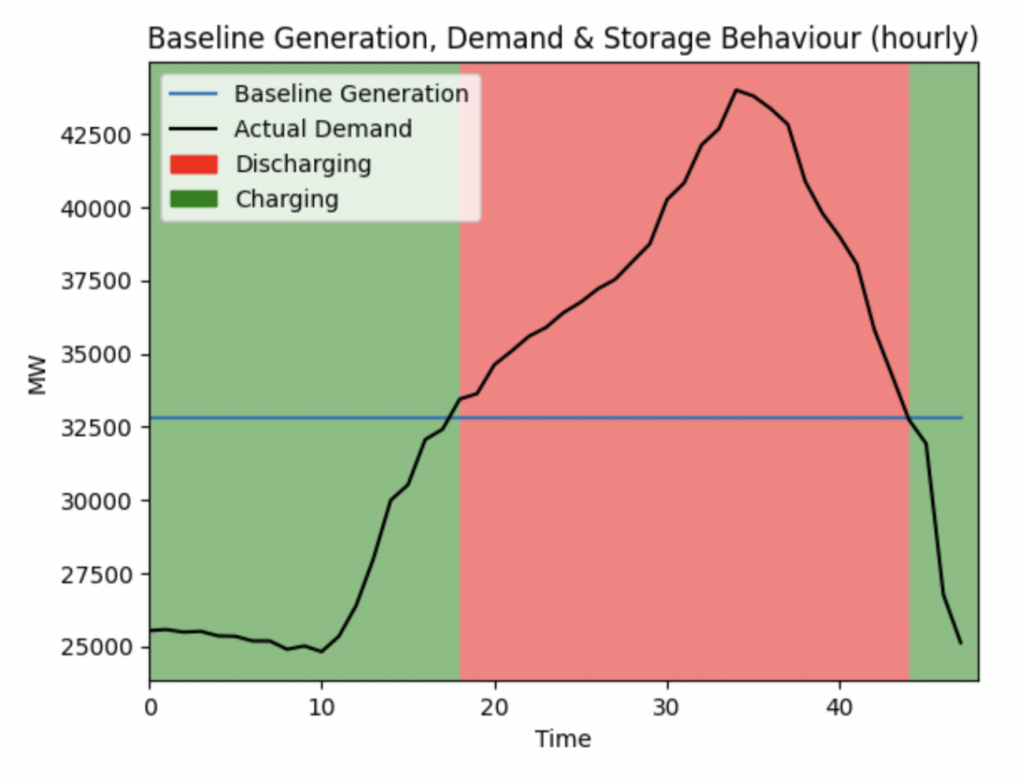
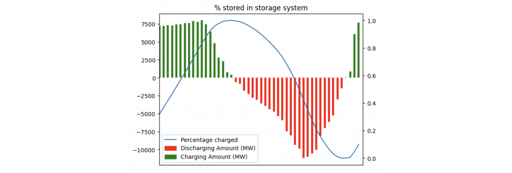
The peak demand for the UK happens during the afternoon, evening and pre-midnight hours. This is when we are discharging as much as possible. Midnight to early noon is when we charge the storage system.
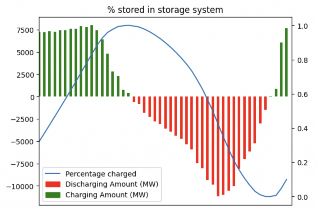
Our storage curve above shows us how this would look
Now we can analyse this and understand the specs for a UK wide energy storage system.
In January, the UK demand is ~1,500 GWh. Our storage capacity is 150 GWh, so about 10% of the total demand. The max charge rate is 8 GW, and the max discharge rate is -10 GW. Armed with these, we can now configure a storage system which could work for the UK.
Takeaways
The toy model works, and we can apply it to real data to understand the requirements for a proper storage system. We now know that a UK wide storage system should store 150 GWh of energy. It also needs to discharge this at a rate of 10 GW per hour.
However, I wanted to end this analysis by adding some randomness to test the robustness of the process.
Using the actual data, I made a quick 7 days forecast, with a random 10% data smear:
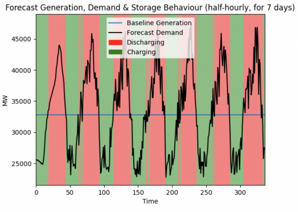
We then apply the same analysis, and can see how the system does:
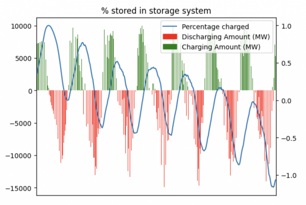
At this level, it falls apart. This can be seen by the storage system going into negative charge after the second discharge cycle. Our predicted baseline was based on the actual data from one day, and doesn’t have a sufficient margin of safety to cover the randomness. A real world system would have more data to drive it and find the right values. However, the exercise is useful in testing the constraints of the model.
From a modelling perspective, this analysis was done using a vectorised approach. This is computationally trivial, but has a few weaknesses. Mainly, a “grid breakdown” just appears as a zero in an array, and isn’t propagated down the system. The behaviour of the system at time t is independent of its behaviour at time t-1. A better way to model this would be an agent based approach, creating a grid agent and seeing how it performs. This approach would also enable us to optimise for certain criteria (carbon intensity, uptime, curtailment rate etc.).
The next posts in this series will cover the different technologies we have for energy storage, the feasibility of building a system which could address the UK’s needs, and an exploration into building an agent-based model to better understand grid dynamics.
If you work in this space and would like to comment, or if you’re an energy storage startup working on this, please connect with me on LinkedIn to get in touch.

